模型压缩——网络量化

Rogerspy

2021-02-25

笔记

字数统计: 2k字 | 阅读时长≈ 10分

1. 理论基础

如果有人问你现在几点了，你不会告诉他现在“10:14:34:4301”，而是会告诉他现在“10:15”。

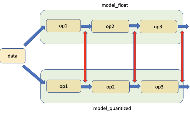
量化就是通过降低网络层权重和/或激活函数的数值精度达到模型压缩的方法。通常神经网络模型的参数都是过量的，将模型进行压缩可以使模型更小，运算速度更快。通常硬件上 8-bit 精度的数据比 32-bit 的数据处理速度更快。

1.1 映射函数

这里所说的映射函数就是将浮点数映射到整型数。一个常用的映射函数为：

$Q(r) = \text{round}(\frac{r}{S}+Z)$

其中 $r$ 是输入，$S,Z$ 分别是量化参数。通过下式可以将量化后的输入进行浮点数翻转：

$\tilde{r} = (Q(r)-Z)\cdot S$

注意 $\tilde{r}\ne r$，两者的差距表示量化误差。

1.2 量化参数

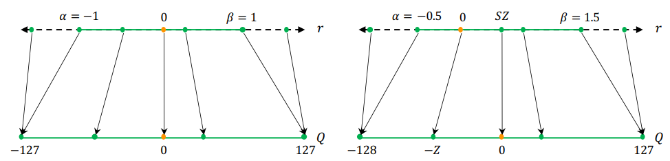
上面我们说到 $S,Z$ 表示量化参数，$S$ 可以简单的表示成输入范围和输出范围的比值：

$S = \frac{\beta-\alpha}{\beta_q-\alpha_q}$

其中 $[\alpha, \beta]$ 表示输入的范围，即允许输入的上下界；$[\alpha_q, \beta_q]$ 表示量化后的输出的上下界。对于 8-bit 来说，输出的上下界为 $\beta_q -\alpha_q \le 2^8-1$。

$Z$ 表示偏差，如果输入中有 0，$Z$ 用来保证将 0 也映射到 0：$Z = -\frac{\alpha}{S}-\alpha_q$。

1.3 校准

选择输入限定范围的过程称之为校准。最简单的方法就是记录输入的最小最大值作为 $\alpha, \beta$。不同的校准方法会带来不同的量化策略。

$\alpha=r_{min},\beta=r_{max}$ 时，称之为非对称量化，因为 $-\alpha\ne \beta$；
$\alpha=-\max(|r_{min}|, |r_{max}|), \beta = \max(|r_{min}|, |r_{max}|)$ 时，称之为对称量化，因为 $-\alpha=\beta$。

在实际应用中，对称量化应用更加广泛，因为其可以令 $Z=0$，这样可以减少推理过程计算成本。而非对称量化比对称量化更加紧凑。非对称量化容易受到异常值的影响，所以可以改进为百分比或者 KL 散度来优化这个问题。

act =  torch.distributions.pareto.Pareto(1, 10).sample((1,1024))
weights = torch.distributions.normal.Normal(0, 0.12).sample((3, 64, 7, 7)).flatten()

def get_symmetric_range(x):
  beta = torch.max(x.max(), x.min().abs())
  return -beta.item(), beta.item()

def get_affine_range(x):
  return x.min().item(), x.max().item()

def plot(plt, data, scheme):
  boundaries = get_affine_range(data) if scheme == 'affine' else get_symmetric_range(data)
  a, _, _ = plt.hist(data, density=True, bins=100)
  ymin, ymax = np.quantile(a[a>0], [0.25, 0.95])
  plt.vlines(x=boundaries, ls='--', colors='purple', ymin=ymin, ymax=ymax)

fig, axs = plt.subplots(2,2)
plot(axs[0, 0], act, 'affine')
axs[0, 0].set_title("Activation, Affine-Quantized")

plot(axs[0, 1], act, 'symmetric')
axs[0, 1].set_title("Activation, Symmetric-Quantized")

plot(axs[1, 0], weights, 'affine')
axs[1, 0].set_title("Weights, Affine-Quantized")

plot(axs[1, 1], weights, 'symmetric')
axs[1, 1].set_title("Weights, Symmetric-Quantized")
plt.show()

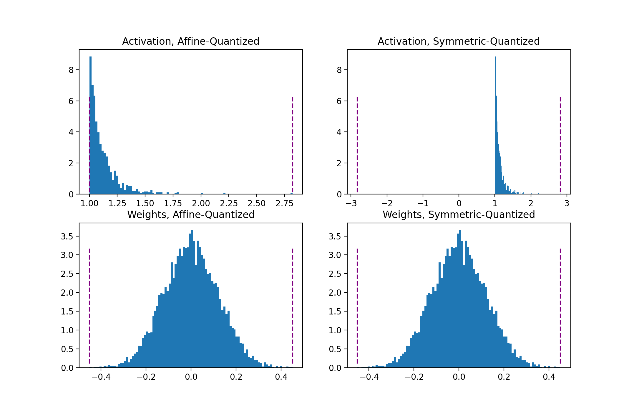
我们可以直接用 Pytorch 内置的模块：

from torch.quantization.observer import MinMaxObserver, MovingAverageMinMaxObserver, HistogramObserver
C, L = 3, 4
normal = torch.distributions.normal.Normal(0,1)
inputs = [normal.sample((C, L)), normal.sample((C, L))]
print(inputs)

# >>>>>
# [tensor([[-0.0590,  1.1674,  0.7119, -1.1270],
#          [-1.3974,  0.5077, -0.5601,  0.0683],
#          [-0.0929,  0.9473,  0.7159, -0.4574]]]),

# tensor([[-0.0236, -0.7599,  1.0290,  0.8914],
#          [-1.1727, -1.2556, -0.2271,  0.9568],
#          [-0.2500,  1.4579,  1.4707,  0.4043]])]

for qscheme in [torch.per_tensor_affine, torch.per_tensor_symmetric]:
  obs = MovingAverageMinMaxObserver(qscheme=qscheme)
  for x in inputs:
      obs(x)
  print(f"Qscheme: {qscheme} | {obs.calculate_qparams()}")

# >>>>>
# Qscheme: torch.per_tensor_affine | (tensor([0.0101]), tensor([139], dtype=torch.int32))
# Qscheme: torch.per_tensor_symmetric | (tensor([0.0109]), tensor([128]))

1.4 Per-Tensor and Per-Channel 量化策略

量化参数可以针对整个权重计算，也可以单独计算每个通道。Per-tensor 就是使用相同的量化参数应用于所有通道，而 per-channel 是不同的通道使用不同的量化参数：

通常权重的量化方面，对称 per-channel 量化效果更好。

from torch.quantization.observer import MovingAveragePerChannelMinMaxObserver
obs = MovingAveragePerChannelMinMaxObserver(ch_axis=0)  # calculate qparams for all `C` channels separately
for x in inputs: obs(x)
print(obs.calculate_qparams())

# >>>>>
# (tensor([0.0090, 0.0075, 0.0055]), tensor([125, 187,  82], dtype=torch.int32))

1.5 QConfig

用 QCfing NameTuple 存储 Observers 和量化策略：

my_qconfig = torch.quantization.QConfig(
  activation=MovingAverageMinMaxObserver.with_args(qscheme=torch.per_tensor_affine),
  weight=MovingAveragePerChannelMinMaxObserver.with_args(qscheme=torch.qint8)
)
# >>>>>
# QConfig(activation=functools.partial(<class 'torch.ao.quantization.observer.MovingAverageMinMaxObserver'>, qscheme=torch.per_tensor_affine){}, weight=functools.partial(<class 'torch.ao.quantization.observer.MovingAveragePerChannelMinMaxObserver'>, qscheme=torch.qint8){})

2. In Pytorch

2.1 Post-Training Dynamic/Weight-only Quantization

import torch
from torch import nn

# toy model
m = nn.Sequential(
  nn.Conv2d(2, 64, (8,)),
  nn.ReLU(),
  nn.Linear(16,10),
  nn.LSTM(10, 10))

m.eval()

## EAGER MODE
from torch.quantization import quantize_dynamic
model_quantized = quantize_dynamic(
    model=m, qconfig_spec={nn.LSTM, nn.Linear}, dtype=torch.qint8, inplace=False
)

## FX MODE
from torch.quantization import quantize_fx
qconfig_dict = {"": torch.quantization.default_dynamic_qconfig}  # An empty key denotes the default applied to all modules
model_prepared = quantize_fx.prepare_fx(m, qconfig_dict)
model_quantized = quantize_fx.convert_fx(model_prepared)

通常会有更高的准确率；
对于 LSTM / Transformer 来说，动态量化是首选；
每一层事实校准和量化可能需要消耗算力。

2.2 Post-Training Static Quantization (PTQ)

# Static quantization of a model consists of the following steps:

#     Fuse modules
#     Insert Quant/DeQuant Stubs
#     Prepare the fused module (insert observers before and after layers)
#     Calibrate the prepared module (pass it representative data)
#     Convert the calibrated module (replace with quantized version)

import torch
from torch import nn

backend = "fbgemm"  # running on a x86 CPU. Use "qnnpack" if running on ARM.

m = nn.Sequential(
     nn.Conv2d(2,64,3),
     nn.ReLU(),
     nn.Conv2d(64, 128, 3),
     nn.ReLU()
)

## EAGER MODE
"""Fuse
- Inplace fusion replaces the first module in the sequence with the fused module, and the rest with identity modules
"""
torch.quantization.fuse_modules(m, ['0','1'], inplace=True) # fuse first Conv-ReLU pair
torch.quantization.fuse_modules(m, ['2','3'], inplace=True) # fuse second Conv-ReLU pair

"""Insert stubs"""
m = nn.Sequential(torch.quantization.QuantStub(), 
                  *m, 
                  torch.quantization.DeQuantStub())

"""Prepare"""
m.qconfig = torch.quantization.get_default_qconfig(backend)
torch.quantization.prepare(m, inplace=True)

"""Calibrate
- This example uses random data for convenience. Use representative (validation) data instead.
"""
with torch.inference_mode():
  for _ in range(10):
    x = torch.rand(1,2, 28, 28)
    m(x)
    
"""Convert"""
torch.quantization.convert(m, inplace=True)

"""Check"""
print(m[[1]].weight().element_size()) # 1 byte instead of 4 bytes for FP32


## FX GRAPH
from torch.quantization import quantize_fx
m.eval()
qconfig_dict = {"": torch.quantization.get_default_qconfig(backend)}
# Prepare
model_prepared = quantize_fx.prepare_fx(model_to_quantize, qconfig_dict)
# Calibrate - Use representative (validation) data.
with torch.inference_mode():
  for _ in range(10):
    x = torch.rand(1,2,28, 28)
    model_prepared(x)
# quantize
model_quantized = quantize_fx.convert_fx(model_prepared)

静态量化比动态量化更快；
静态量化模型可能需要定期重新校准以保持对分布漂移的鲁棒性。

2.3 Quantization-aware Training (QAT)

# QAT follows the same steps as PTQ, with the exception of the training loop before you actually convert the model to its quantized version

import torch
from torch import nn

backend = "fbgemm"  # running on a x86 CPU. Use "qnnpack" if running on ARM.

m = nn.Sequential(
     nn.Conv2d(2,64,8),
     nn.ReLU(),
     nn.Conv2d(64, 128, 8),
     nn.ReLU()
)

"""Fuse"""
torch.quantization.fuse_modules(m, ['0','1'], inplace=True) # fuse first Conv-ReLU pair
torch.quantization.fuse_modules(m, ['2','3'], inplace=True) # fuse second Conv-ReLU pair

"""Insert stubs"""
m = nn.Sequential(torch.quantization.QuantStub(), 
                  *m, 
                  torch.quantization.DeQuantStub())

"""Prepare"""
m.train()
m.qconfig = torch.quantization.get_default_qconfig(backend)
torch.quantization.prepare_qat(m, inplace=True)

"""Training Loop"""
n_epochs = 10
opt = torch.optim.SGD(m.parameters(), lr=0.1)
loss_fn = lambda out, tgt: torch.pow(tgt-out, 2).mean()
for epoch in range(n_epochs):
  x = torch.rand(10,2,24,24)
  out = m(x)
  loss = loss_fn(out, torch.rand_like(out))
  opt.zero_grad()
  loss.backward()
  opt.step()

"""Convert"""
m.eval()
torch.quantization.convert(m, inplace=True)

QAT 准确率比 PTQ 高；
量化参数可以随着模型一起训练；
QAT 的模型重训可能需要消耗不少时间。

3. 灵敏度分析

并不是所有层在量化中起到的作用都是相等的，有些层对准确率的影响可能会比较大，要想找出最优的量化层与准确率的解是比较消耗时间的，所以人们提出使用 one-at-a-time 方法来分析那些层对准确率最敏感，然后再 32-bit 浮点数上重训：

# ONE-AT-A-TIME SENSITIVITY ANALYSIS 

for quantized_layer, _ in model.named_modules():
  print("Only quantizing layer: ", quantized_layer)

  # The module_name key allows module-specific qconfigs. 
  qconfig_dict = {"": None, 
  "module_name":[(quantized_layer, torch.quantization.get_default_qconfig(backend))]}

  model_prepared = quantize_fx.prepare_fx(model, qconfig_dict)
  # calibrate
  model_quantized = quantize_fx.convert_fx(model_prepared)
  # evaluate(model)

Pytorch 停工了分析工具：

# extract from https://pytorch.org/tutorials/prototype/numeric_suite_tutorial.htmlimport torch.quantization._numeric_suite as nsdef SQNR(x, y):    # Higher is better    Ps = torch.norm(x)    Pn = torch.norm(x-y)    return 20*torch.log10(Ps/Pn)wt_compare_dict = ns.compare_weights(fp32_model.state_dict(), int8_model.state_dict())for key in wt_compare_dict:    print(key, compute_error(wt_compare_dict[key]['float'], wt_compare_dict[key]['quantized'].dequantize()))act_compare_dict = ns.compare_model_outputs(fp32_model, int8_model, input_data)for key in act_compare_dict:    print(key, compute_error(act_compare_dict[key]['float'][0], act_compare_dict[key]['quantized'][0].dequantize()))

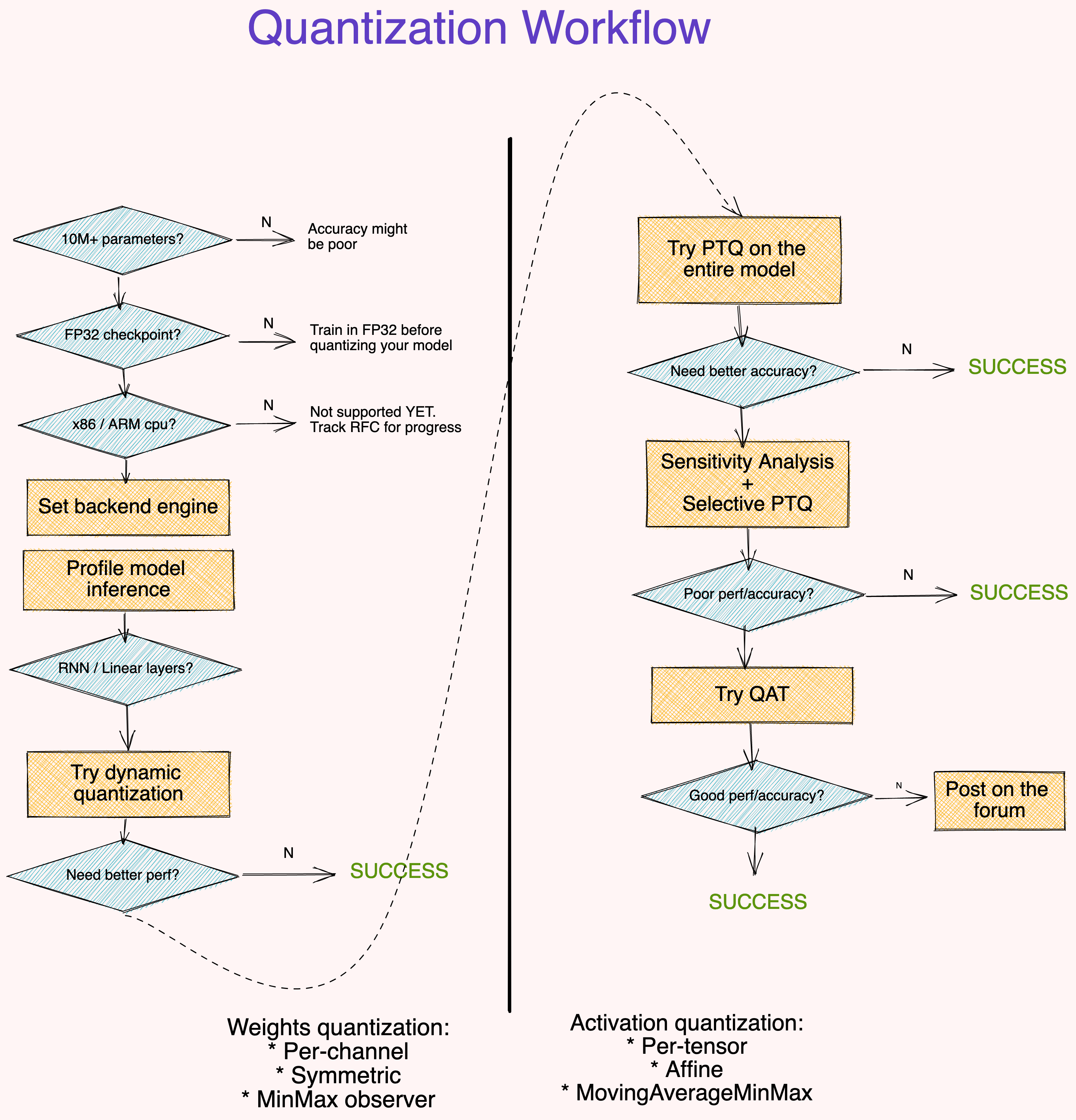
4. 模型量化工作流

5. 写在最后

大模型（参数量大于 1 千万）对量化误差更鲁棒；
从 FP32 开始训练模型比 INT8 开始训练模型准确率更高；
如果模型中有大量的线性层或者递归层，可以首先考虑动态量化；
用 MinMax 对称 per-channel 量化权重，用 MovingAverageMinMax 非对称 per-tensor 量化激活函数。

Reference

Practical Quantization in PyTorch